RandomForestClassifier Algorithm in ML

In this exercise, we will learn about the RandomForestClassifier Algorithm in the ML.

Random Forest Classifier Algorithm The Random Forest Classifier is an ensemble learning method primarily used for classification (and regression) tasks. It is based on constructing multiple decision trees during training and outputs the class that is the mode of the classes predicted by individual trees.

Example: Implementing Random Forest in Python Let’s see how we can use the RandomForestClassifier from the sklearn library.

In this exercise, we will use the data.csv file as the data source for training the machine learning algorithm. You can also download this data and use it for the ML task.

Importing Necessary Libraries

Python

import numpy as np
import pandas as pd

Load the data into the pandas dataframe.

Python

# Load Data into Pandas DataFrame
# df = pd.read_csv("file_path")
df = pd.read_csv("data.csv")
df

The output of the above code is shown below:

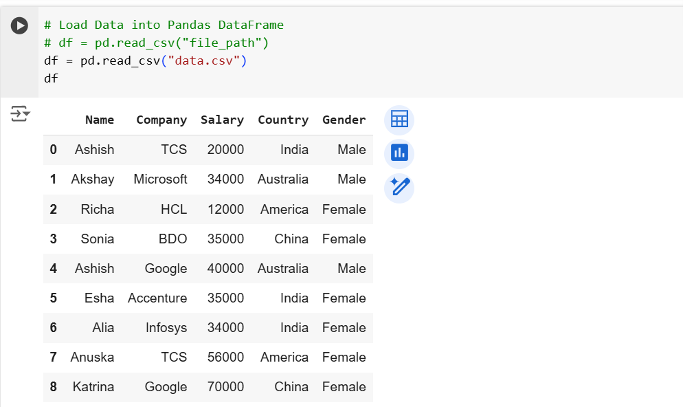
Let’s get the count of Males and Females in the Dataframe.

Python

df["Gender"].value_counts()

The output of the above code is shown below:

We found that there are 6 Females and 3 Males in the source data. So, we extract the Male data in one variable named minority and Female data in one variable named majority.

Python

minority = df[df['Gender'] == "Male"]
majority = df[df['Gender'] == "Female"]

We are going to do resampling in the data so number of males and females in the data is equal, so there is no gender bias in the trained model.

Python

from sklearn.utils import resample
minority_upsampled = resample(minority, replace=True, n_samples=len(majority), random_state=42)
minority_upsampled

The output of the above code is shown below:

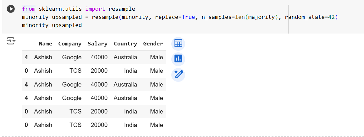
Now we are going to concat the majority and minority_upsampled data.

Python

df_balanced = pd.concat([majority, minority_upsampled])
df_balanced

The output of the above code is shown below:

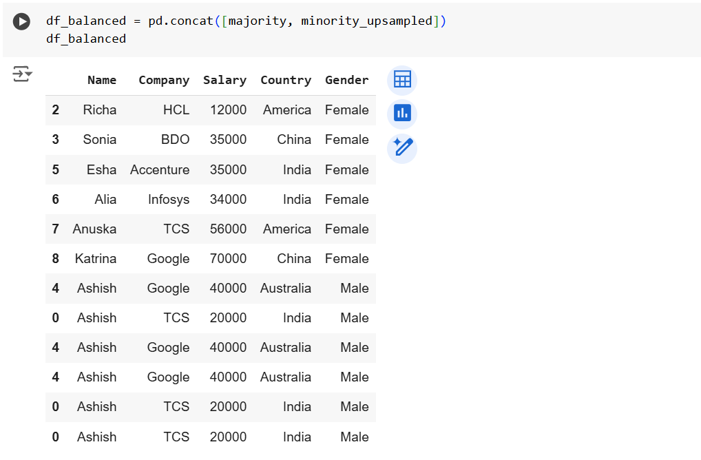
Let’s again check the number of Males and Females in the transformed data.

Python

df_balanced['Gender'].value_counts()

The output of the above code is shown below:

So, now we can see 6 Female and 6 Males.

We have a column Company which are going to use in the machine learning, to use it we need to convert the values in some numerical value. To do so, we can use the get_dummies pandas function.

Python

df_encoded = pd.get_dummies(df_balanced, columns=['Company'], dtype=int)
df_encoded

The output of the above code is shown below:

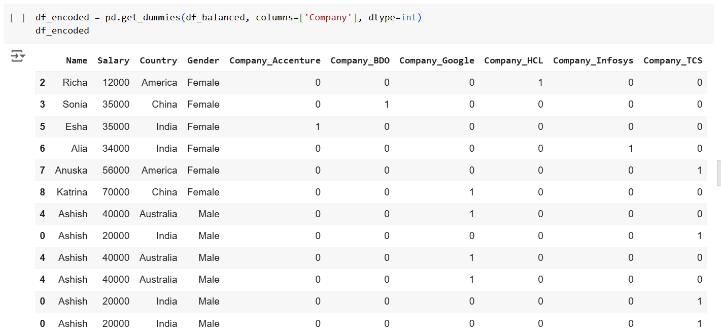
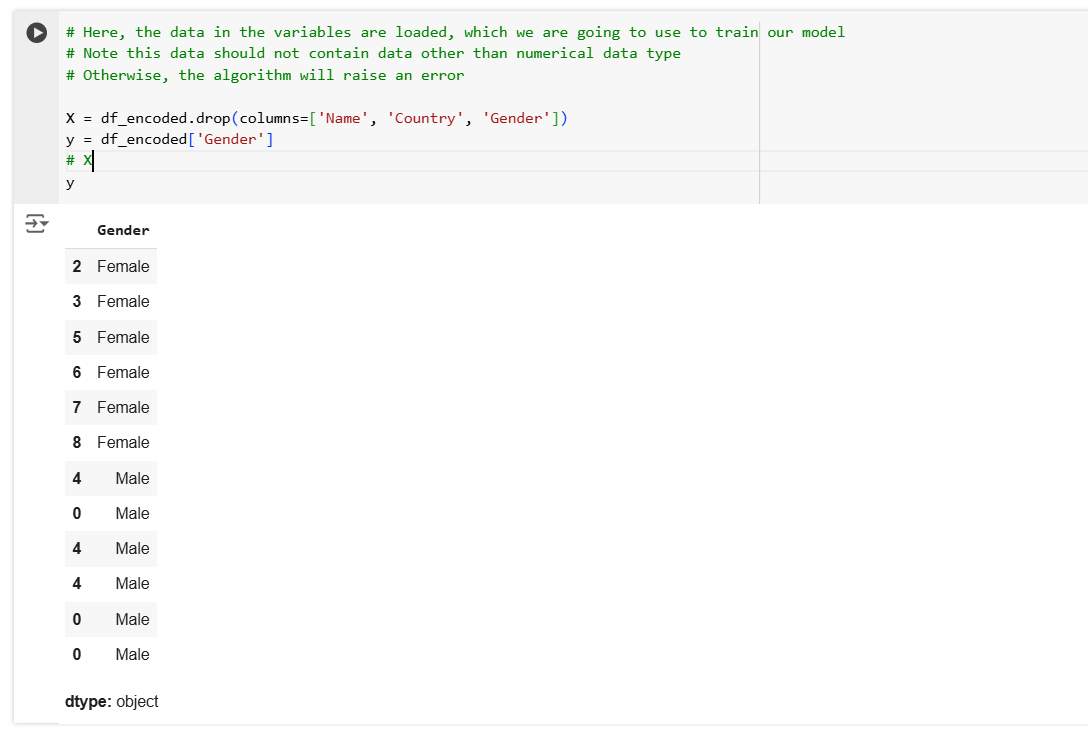
Now we are selecting the columns from the transformed data for the features and target value in the X and y variables.

Python

# Here, the data in the variables are loaded, which we are going to use to train our model
# Note this data should not contain data other than numerical data type
# Otherwise, the algorithm will raise an error

X = df_encoded.drop(columns=['Name', 'Country', 'Gender'])
y = df_encoded['Gender']
X

The output of the above code is shown below:

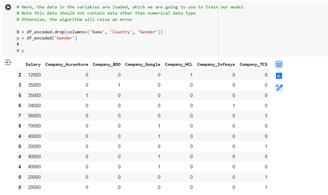
And in the y variable we have the data as shown below:

Now it’s time to split the training and testing data. Here we are using the 60% data for training and 40% for testing.

Python

# import the module
from sklearn.model_selection import train_test_split

# Split the dataset into training and testing sets
X_train, X_test, y_train, y_test = train_test_split(X, y, test_size=0.4, random_state=42)

The train_test_split function is from the sklearn.model_selection module and is used to split a dataset into training and testing sets.

The following are the parameters in the function:

X: Feature matrix (independent variables or predictors).
y: Target vector (dependent variable or labels).
test_size=0.4: Specifies the proportion of the dataset to include in the test split (40% of the data for testing, 60% for training in this case).
random_state=42: Ensures reproducibility by setting a seed for the random number generator. This guarantees the same split each time the code runs.

In the output, the function returns:

X_train: Training set features (60% of X).
X_test: Test set features (40% of X).
y_train: Training set labels corresponding to X_train.
y_test: Test set labels corresponding to X_test.

The names X_train, X_test, y_train, and y_test are just standard convention names, but we can use any variable names that make sense for our application.
For example, you can write:

Python

features_train, features_test, labels_train, labels_test = train_test_split(X, y, test_size=0.4, random_state=42)

Here, the variables are renamed to:

features_train for the training features.
features_test for the testing features.
labels_train for the training labels.
labels_test for the testing labels.

Now train the model using the training data with RandomForestClassifier model algorithm.

RandomForestClassifier We can initialize the algorithm using the below syntax. Syntax model = RandomForestClassifier(n_estimators=100, random_state=42)

The parameter n_estimators has the default value 100. It specifies the number of trees in the forest.

Python

# Training the Random Forest Classifier

# Import the module
from sklearn.ensemble import RandomForestClassifier

# Initialize the classifier
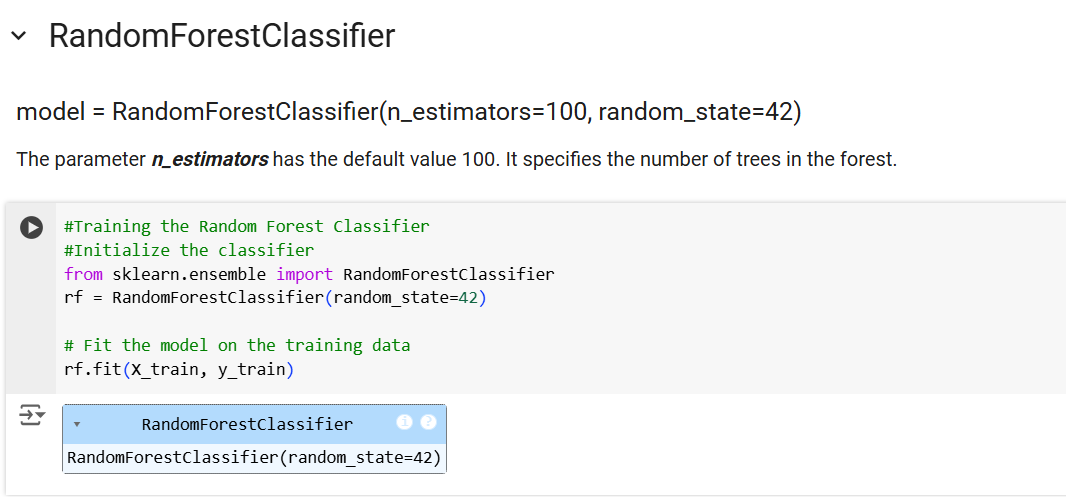
rf = RandomForestClassifier(random_state=42)

# Fit the model on the training data
rf.fit(X_train, y_train)

The output of the above code is shown below:

Now it's time to make the predictions on the testing data.

Python

# Make predictions on the test set
y_pred = rf.predict(X_test)
y_pred

The output of the above code is shown below:

Now we are evaluating the model.

Python

# import the module
from sklearn.metrics import classification_report

# Generate the classification report
report = classification_report(y_test, y_pred)

# print the classification report
print("Classification Report:\n", report)

The output of the above code is shown below:

Q: What is a Classification Report? A Classification Report is a detailed performance evaluation tool provided by the scikit-learn library in Python. It summarizes the key metrics used to assess the effectiveness of a classification model, helping you understand how well your model is performing on each class.

The classification report includes:

Precision
Recall (Sensitivity)
F1 Score
Support

These metrics are calculated for each class in your dataset and provide a deeper insight than just looking at accuracy, especially for imbalanced datasets.

Key Metrics Explained Here's what each metric in the classification report represents: 1. Precision:

The proportion of correctly predicted positive observations to the total predicted positives.
Formula: Precision=TP/(TP+FP)
High precision indicates a low false positive rate.

2. Recall (Sensitivity or True Positive Rate):

The proportion of correctly predicted positive observations to all actual positives.
Formula: Recall=TP/(TP+FN)
High recall indicates a low false negative rate.

3. F1 Score:

The harmonic mean of precision and recall. It balances the two, especially useful when you need a single metric to compare models.
Formula: F1=(2×Precision×Recall)/(Precision+Recall)
A high F1 score indicates both high precision and recall.

4. Support:

The number of actual occurrences of each class in your dataset.
This is not a performance metric but rather a count of the samples available for each class.

Previous Next