Pivot columns in Power Query Editor in Power BI

In Power Query Editor, we can create the multiple columns in the table by using the column values of a single value.

To pivot a column, follow the following steps:

Step 1: Let’s we have the following table in Power BI.

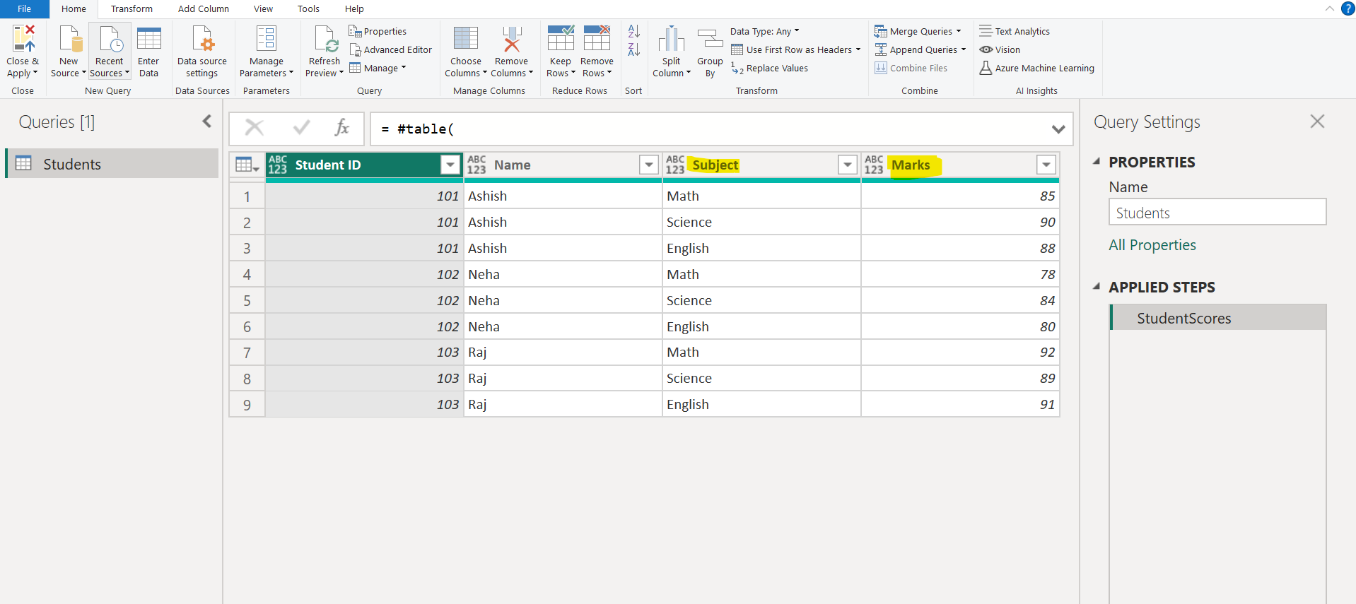
We can use the below M code to create the table:

Example: Creating a table of student scores across subjects.

Power Query M

let
    StudentScores = #table(
        {"Student ID", "Name", "Subject", "Marks"},
        {
            {101, "Ashish", "Math", 85},
            {101, "Ashish", "Science", 90},
            {101, "Ashish", "English", 88},
            {102, "Neha", "Math", 78},
            {102, "Neha", "Science", 84},
            {102, "Neha", "English", 80},
            {103, "Raj", "Math", 92},
            {103, "Raj", "Science", 89},
            {103, "Raj", "English", 91}
        }
    )
in
    StudentScores 

This code creates a table named StudentScores containing student IDs, names, subjects, and marks for three subjects.

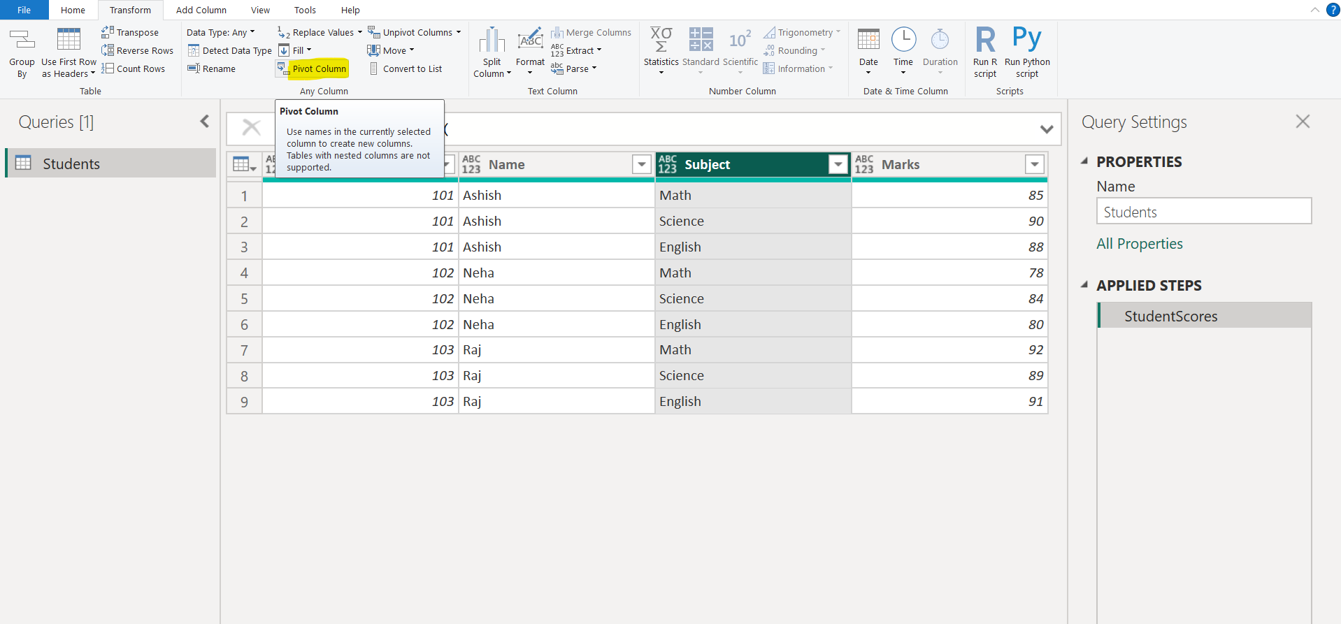
Step 2: Select the column that we want to pivot, and then on the Transform tab in the Any column group, select Pivot column.

Step 3: In the Pivot column dialog box, in the “Values column” list, select Marks.

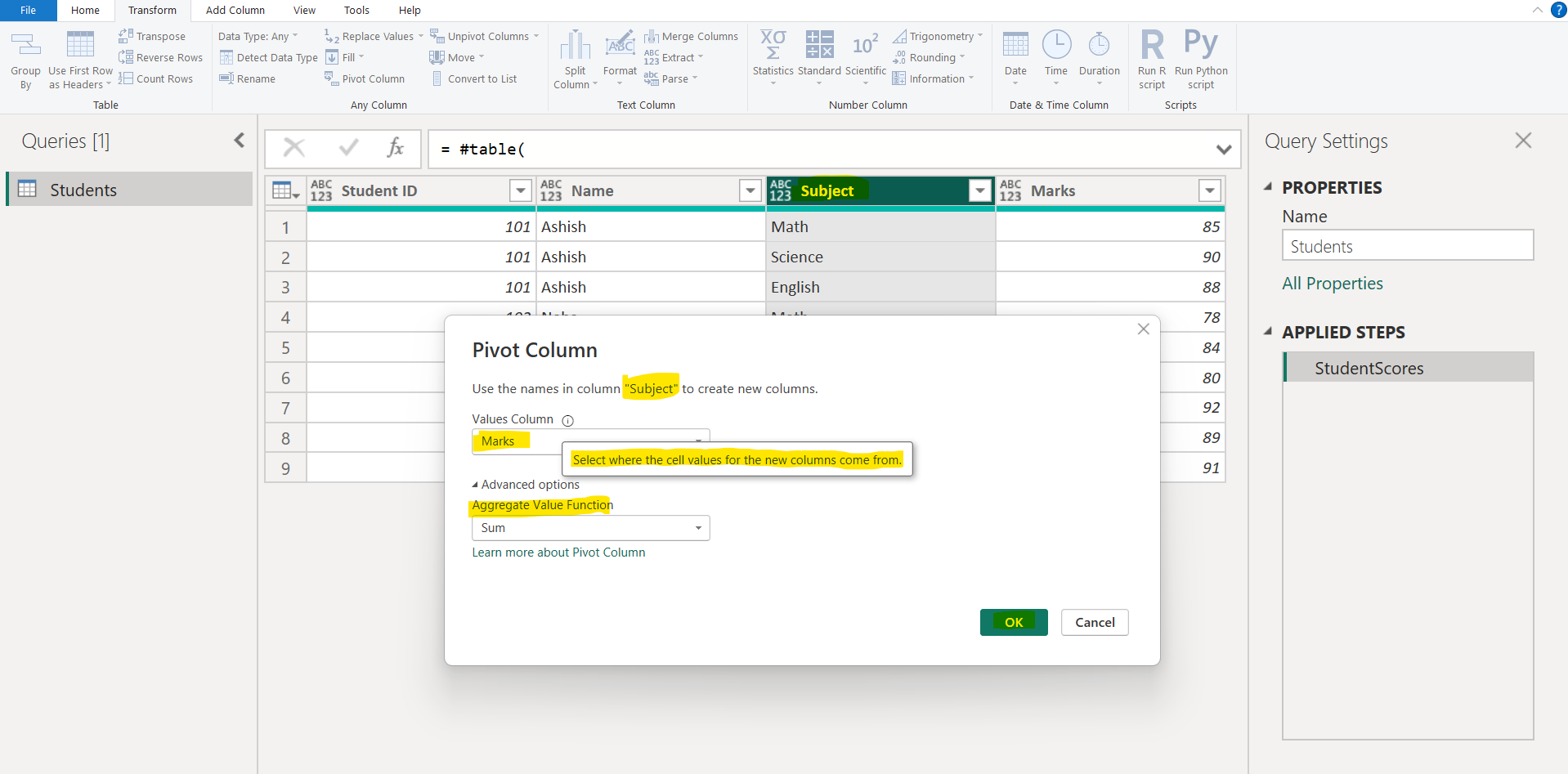
We can see also in the dialog it is written there, “Use the names in column “Subject” to create new columns.”

In the “Values Column” dropdown, it contains a list of columns, from which we can decide the cell value to come from for pivot columns.

In the “Aggregate Value Function” we can specify the aggregation method to use when we have multiple values for the same row. By default, Power Query will try to do a sum as the aggregation for numeric columns, but we can select other available aggregations.

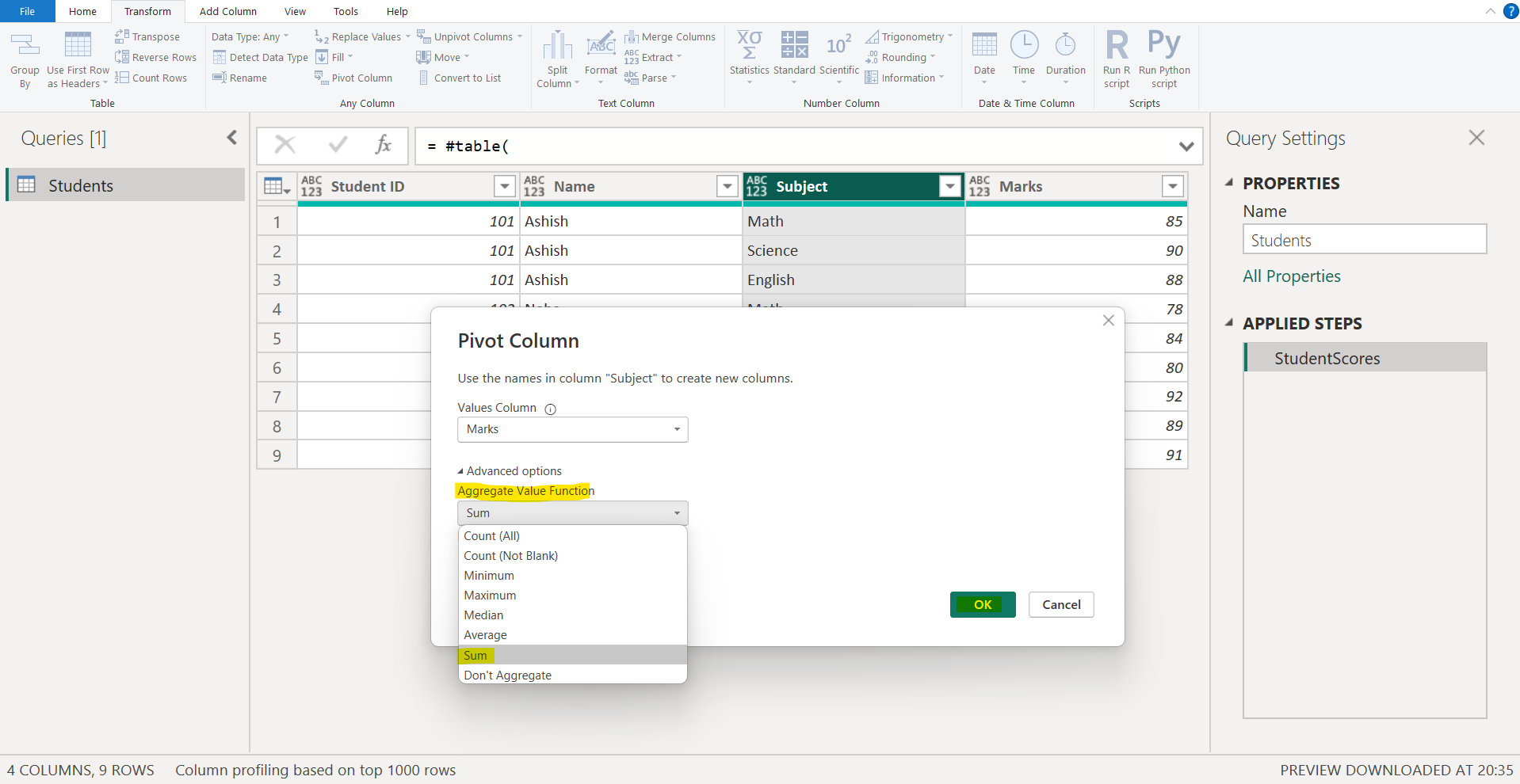
Available aggregation options:

• Don't Aggregate
• Count (All)
• Count (Not Blank)
• Minimum
• Maximum
• Median
• Sum
• Average

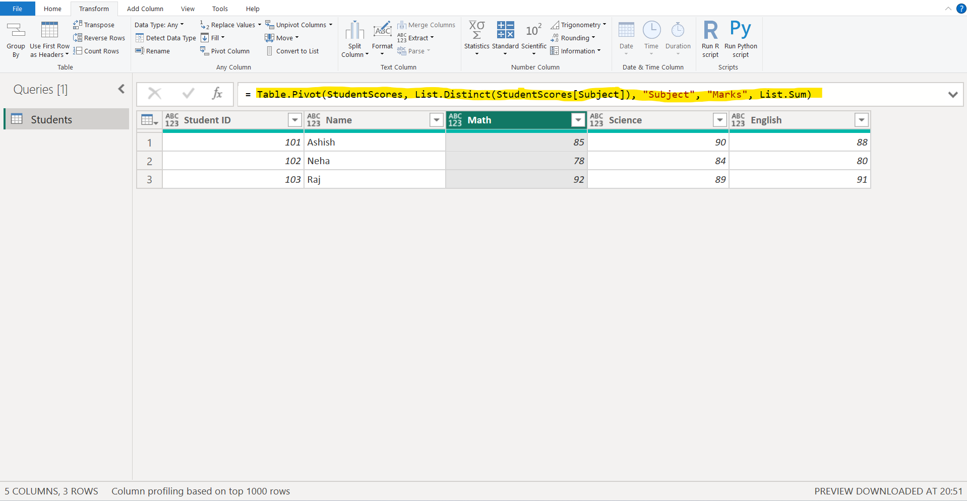
After selecting the desired option, click OK. The result of this operation will be displayed as shown in the following image.